Digital Audio
Sound hits our ears in unbroken waves. Air compresses and rarefies smoothly. Analog signals - like my voice for example - can be represented digitally by using a sensitive membrane connected to a transducer - aka a microphone - to sample these changes in pressure at a regular interval - this is the sampling rate.
Sampling Signals
The principle is the same when sampling from an analog audio signal, like the headphone output from an FM radio. The analog signal is a continuous voltage - just like the signal produced by the transducer in a microphone - you could pick any tiny point in time, and if you had good enough instruments, measure the value of the signal, and be able to track the tiniest of changes in the shortest intervals.
Once the audio has been sampled, what we actually have is a collection of numbers - specifically integers of a certain type - representing each instananious value of the signal. The range of these integers correlates to the dynamic range of the audio.
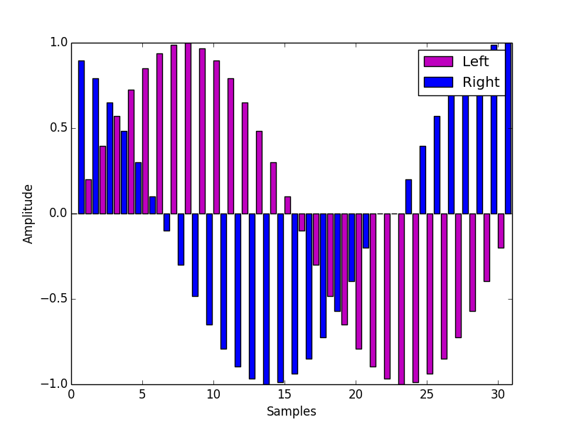
A stream of interleaved stereo audio samples. A sinewave was sampled in each channel at a different phase.
Dynamic Range
Lets say our range is between -100 and 100. If the speaker cone is pushed all the way out, the value is 100. If it is pulled all the way in, the value is -100. If it is at rest (and therefore silent) the value is 0. This means we have exactly 201 possible amplitudes to work with. (That extra 1 comes from the 0 value.)
This range doesn’t affect absolute loudness - that is to say, if we had a range of -200 to 200, the audio would not be twice as loud, but we would have almost twice the number of choices for amplitudes.
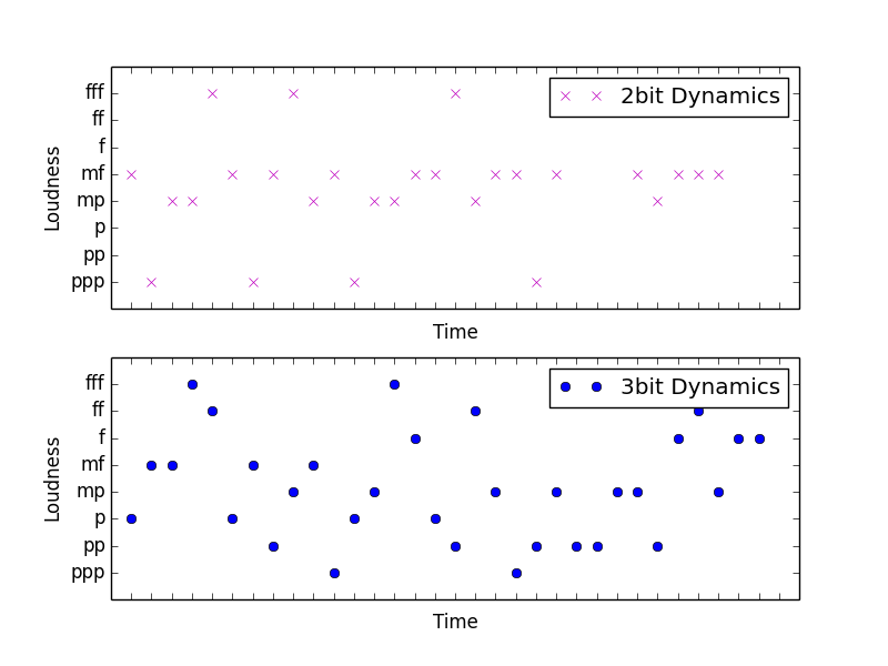
If we were writing music with western notation and we were limited to ppp, mp, mf, and fff
for dynamic markings, this would be the equivelant to working with a low bit depth in digital audio.
If we then wrote music using ppp, pp, p, mp, mf, f, ff, fff, and fff for dynamic
markings, we haven’t changed the absolute loudness of the music, but we’ve given ourselves more
dynamic range.
The same is true for digital audio, but there are different consequences to audio with a limited bit depth.
Bit Depth & Binary Integers
Before I get into that, lets touch on why the dynamic range of digital audio is described in terms of bit depth. Earlier I mentioned that when we sample audio, what we actually end up is a collection of integers of a specific sort. What sort exactly depends precisely on the bit depth of the audio we’re targeting. Computers store integers - and every other thing! - as a series of 1s and 0s as you probably know.
Each of those 1s or 0s is called a bit. If we only needed to store 2 possible values, we could just use a single bit. So, the number 1 would be:
1
How about the number 3? We need to add a bit to give us more possible values. Using two bits, here is our 1 again:
0 1
The farthest bit to the right (this is called little-endian format fwiw, in reverse it’s big-endian) is the ones column - so 0 is 0 and 1 is 1 - but our new bit is the twos column: 0 is 0 and 1 is 2.
To store a three in binary, we’d write these bits into the computer’s memory:
1 1
Adding it up from left to right, we have a value of 2 and a value of 1, and now we have our 3!
Using two bits to store each sampled number in a digital audio stream means we would have a bit depth of 2, and exactly 4 possible dynamics for our audio.
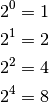
And how about 9? Add two more bits. These will represent the 4s and 8s columns - because this is a base 2 system, each additional bit is 2 to the power of its column index. So counting from 0 from the right to the left, lowest to highest:
That means we can store nine by setting 4 bits like this:
1 0 0 1
Five: 1 eight plus 0 fours plus 0 twos plus 1 one.
Now we’re working with 4 bit numbers!
Quantization Noise
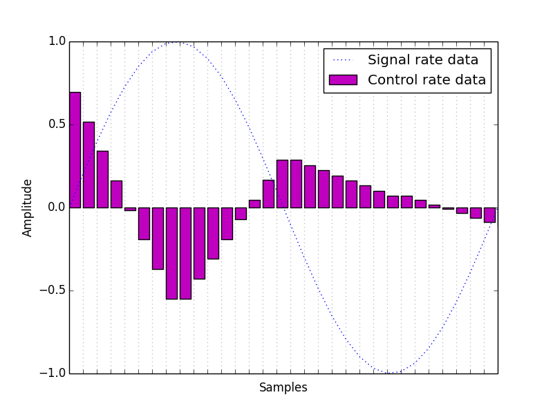
Okay, we can finally get to pure data. Lets listen to how 4 bit audio sounds by sampling my voice with pure data using only the 8 possible values in a 4 bit integer. Here’s a graph of what a sinewave recorded at this bit depth would look like:
[ graph ]
You can see discontinuities where the audio makes huge jumps between values. As a general rule, sounds with rougher and more angular shapes have a richer timbre, with more energy in the upper partials. These jumps are just about as extreme as you can get in digital audio, so at those moments of transition the sound has a lot of energy across the frequency spectrum. This is known as quantization noise.
Data in Pure Data
I think one of the most difficult hurdles to leap during the initial learning curve with pure data is learning to understand how it handles and understands data in your patches. Initial frustrations can often be traced back to questions related to data flow - for example:
- How does information flow around the program?
- What different kinds of information are there?
- How does each kind of information behave?
- How do I convert one kind of information into another kind?
The next sections cover some of these cases, but also try to provide the tools to help you discover the answers to these questions on your own when they pop up in unfamiliar places.
Objects and Abstractions
The basic building block in pd is the object. Objects are very much like little highly specialized software guitar pedals. Some objects come with pd itself. If you downloaded the ‘vanilla’ version of pd, you will have a more minimal but very powerful set of objects. If you downloaded Pd extended, you will get a number of additional libraries of objects as well. You can download additional objects that other people have made and use them alongside the built in objects. You can also use your own patches as abstractions - which behave as though they were themselves objects. We’ll come back to that later. First lets start patching.
Inlets, Outlets and Data Types
Objects have inputs and outputs, which you can connect to one another to create a signal path, or send messages. If we wanted to mimic the signal path of a guitar plugged into a volume pedal, which is in turn plugged into an amplifier, in pure data we could create a simple patch with three objects.
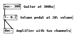
It doesn’t sound much like a guitar, but you can imagine this simple patch as being like a guitarist plugging his guitar into a volume pedal, and the volume pedal into a stereo amplifier.
As the guitar, we can start with an [ osc~ 300 ] object. From the ‘put’ menu, select ‘create object’.
[ osc~ ] and [ dac~ ] are both signal rate objects. Every signal rate object has a tilde at the end of
its name by convention. Signal rate objects do their work very fast. Their speed correlates to the sampling
rate you’ve chosen for your soundcard. Lets assume we’re using a sampling rate of 44,100 samples every second, and a bit depth of
16 bits - in other words, cd quality audio.
In pd the the amplifier at the end of the signal chain is the [ dac~ ] object. (There are other ways to get data in and
out of pd - but for the purposes of this workshop I’ll stick to audio.) The [ dac~ ] object is an interface to your audio
hardware. It has up to as many inlets as your soundcard has channels - so typically there are two inlets: one for the left
channel and one for the right.
Sampling & Signal Rate Objects
Sampling is a concept that will constantly come up in working with digital audio. In different contexts it has specific meanings and can sometimes be confusing, but the basic concept is very simple. Sampling is the process of picking a number out of a stream of numbers in order to represent that stream at a given point in time. In other words, it is a representation of a signal at a certain time.
The sampling rate for an audio system then just tells us how many samples the system will take in one second. Given the settings we decided on for the guitar example above, we could guess that every 1/44100th of a second a signal rate pd object would get a new number in one of its inlets, do something with it, and spit a new number out to one of its outlets. Actually, computation happens in small blocks of numbers. You can change the size of this block, but the default is usually 64 samples. So every 64/44100ths of a second - or about 1.45 milliseconds - pure data will process a block of 64 samples and schedule them for playback. (Miller97, PdMemoryModel) During that 64 sample block, the entire signal chain is calculated. Signal rate objects are constantly being evaluated as long as DSP is on in pd.
While the DAC is on, every 1.45 milliseconds, pd figures out the next 64 values it should send to the [ dac~ ] all at once.
Control rate messages change on every DSP block.
Control Rate Objects
Lets add some GUI objects so we can control our patch interactively. The [ hslider ] and [ vslider ] objects are sliders you
can drag with the mouse to send the corresponding value in a given range to the slider’s outlet. To make this volume pedal [ *~ ]
object more like a volume pedal, we have to have a way to change its value whenever we want. One way to do this is with an [ hslider ]
GUI object.

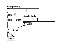
Adding a couple [ hslider ] s and number boxes for interactivity.
Try using the mouse to change the amplitude hslider very fast. The zippering sound you hear is the result of the same
type of discontinuity we saw with quantization noise. Control rate objects only update once every DSP tick - in this case
every 1.45ms - and so the [ *~ ] will hold its value for the duration of each 64 sample tick, and jump to the currently
sampled value from the [ hslider ] on each subsequent tick.
Zipper noise with control rate driven signal objects.
The rest of this workshop will build on and continue to revisit the fundementals touched on above, but now we’re going to get into practical examples of use and build a little software instrument together.
Adc~ and recording into buffers
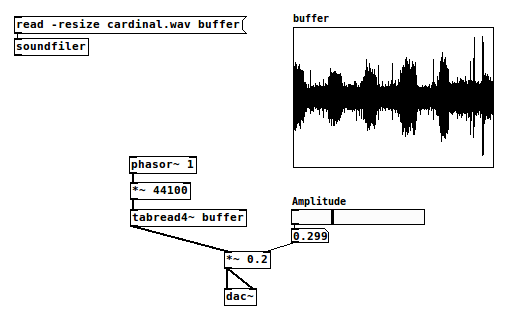
Instead of a sinewave, lets play back a recording. First, use the put menu to create a new array and call it buffer. We’ll use the array to store every sample of the recording we want to play. Don’t worry about the size right now, we’ll resize it in a moment when we load the recording.
Delete the [ osc~ ]] object and replace it with a [ phasor~ 1 ] connected to
a [ *~ 44100 ] object, in turn connected to a [ tabread4~ buffer ] object.
Now, use the put menu to create a new message box and type this into it:
read -resize cardinal.wav buffer
Loading a Sound Into an Array
Connect that to the inlet of a new [ soundfiler ] object. The read message tells
soundfiler you want to read audio from a file into a array. -resize tells it to resize
the array to match the number of samples in the audio file you’re reading from. The next
argument is the filename, which is relative to the patch you’re running. This file is
included in the github repository along with the pure data patches shown in this document.
The final message tells soundfiler which array to write the audio into - in this case, the
buffer array we created earlier. Click the message box to send its contents to the soundfiler
inlet.
Reading audio from a array with tabread4~
Playing Audio From Arrays
Except for soundfiler and the message box, these are all signal rate objects, just like
[ osc~ ] and connect easily to the signal inlet of the [ *~ 0.2 ] object.
*~ will multiply an incoming value (which is always sent to the left inlet) with
the value given as an argument, or a value sent into its right inlet. So far we’ve used
it to attenuate a signal by multiplying it with a value less than 1 and thus created a
handy volume control. Now, we’re taking the stream of values coming out of [ phasor~ ]
and essentially scaling the range of those values by multiplying every value by the sampling
rate, 44100. [ phasor~ 1 ] will output a linear ramp from 0 to 1
at a speed of 1hz - since we gave it an argument of 1. That means we have a nice counter
moving from 0 to 1 over the course of 1 second. We can read through the values stored in our
buffer array by connecting the phasor to a [ tabread4~ ] object. Tabread4~ takes a signal
in its left inlet as an index in the array to read from, and outputs the value in the array
at that index through its outlet.
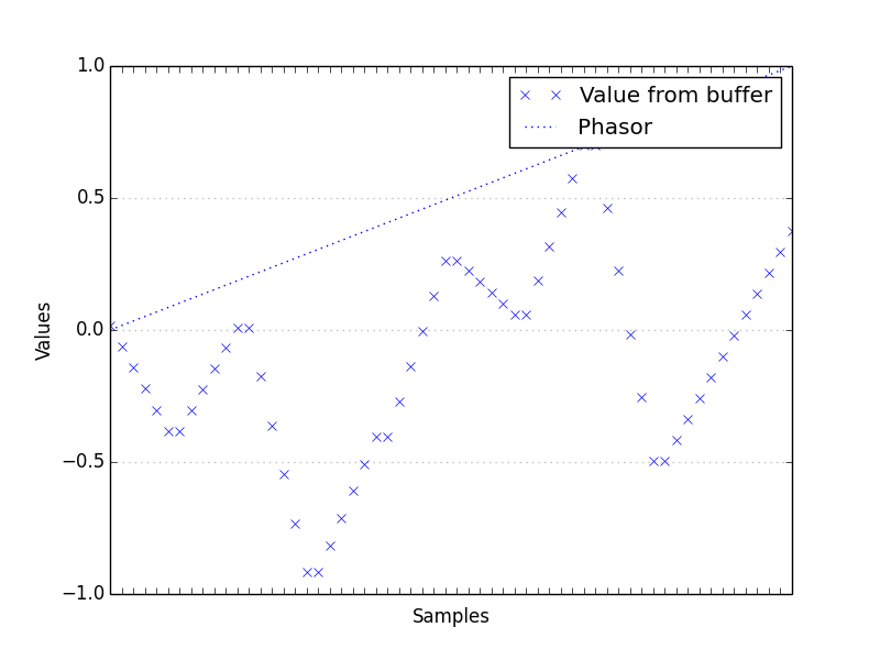
A phasor used as an index to look up values in a buffer
Signal math - relating playback speed to playback range & using it for pitch shifting
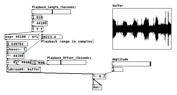
Using control rate objects to calculate playback speeds
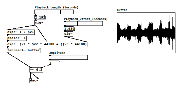
Shorthand signal math with expr~
Using control rate objects to calculate playback speeds
Tidy up patches with s/r/s~/r~/throw~/catch~ and routing
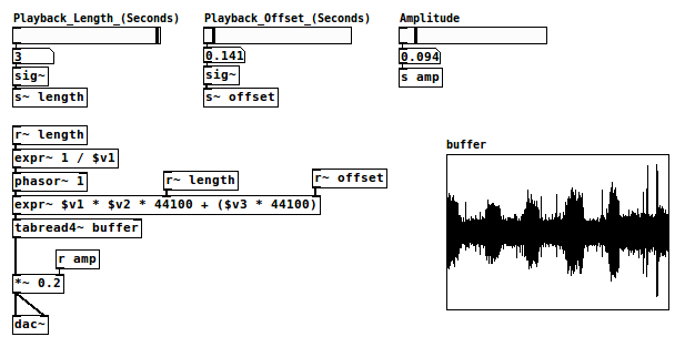
Using s~/r~ and s/r to route data and automatically document your code
Create random numbers with random and expr
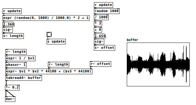
Two methods of generating random ranges of numbers at control rate
Create random numbers with noise~, samphold~, expr~ and phasor~
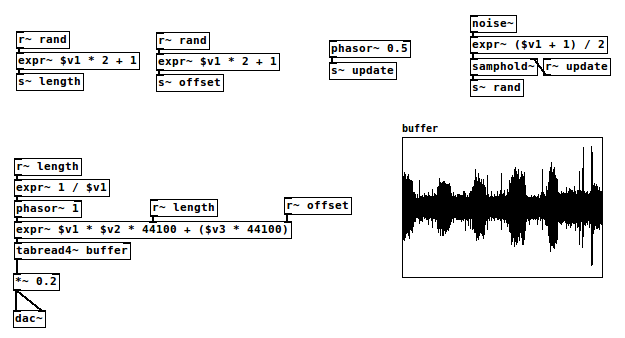
Using samphold~ as a periodic random number generator driven by noise~
Simplify the patch with abstractions
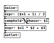
A small signal rate random number generator
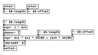
A fairly general purpose buffer playback abstraction
Reducing clutter and improving modularity with abstractions
buffer cosinesum 512 0.1 1.0 0.6

buffer sinesum 512 0.1 1.0 0.6
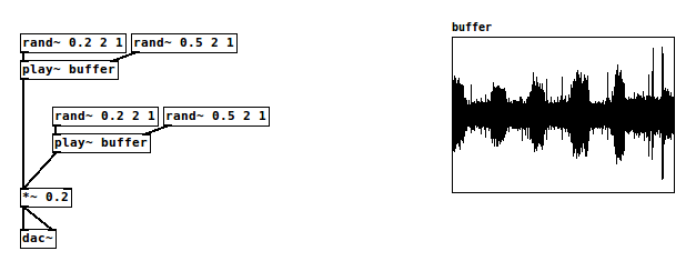
Advanced buffer playback - basic granular techniques
Abstractions and arguments - grain playback objects
Resources
- http://puredata.info The official site. Download PD here and find tons of links to patches and documentation.
- http://puredata.hurleur.com The PD forum. A great place to ask questions, share patches, and generally nerd out about PD.
- http://en.flossmanuals.net/pure-data/ Probably the most readable overview of Pure Data out there, this open source book is always being updated and expanded.
- http://pd-la.info/pd-media/miller-puckette-mus171-videos/ A full introductory course on creating computer music with pure data taught by the author of pure data.
Citations
| [Miller97] | http://puredata.info/docs/articles/puredata1997 |
| [PdMemoryModel] | http://puredata.info/docs/developer/PdMemoryModel/view |